Automatic differentiation in RooFit with Clad

Maybe you have heard that RooFit now supports Automatic Differentiation (AD) for faster likelihood minimization. This blogpost explains you the underlying technology, implementation, and interfaces. It also showcases some performance numbers from a Higgs analysis benchmark before concluding with an outlook on future developments.

This blogpost is quite extensive, deep-diving into everything that I think is worth knowing about this subject for any RooFit user.

Introduction to Automatic differentiation with Clad

Analytic derivatives with Clad

Did you know that ROOT can do Automatic Differentiation (AD) of mathematical C++ functions using the built-in Clad compiler plugin?

Here is a simple example on how to create an automatic derivative with Clad in ROOT:

#include <Math/CladDerivator.h>

double f(double x, double y) { return x * x * y; }

// Call clad to generate the derivative of f wrt x.
auto f_dx = clad::differentiate(f, "x");

// Execute the generated derivative function.
std::cout << "f_dx(3, 4) = << " f_dx.execute(/*x=*/3, /*y=*/4) << std::endl;

// Dump the generated derivative code to standard output.
f_dx.dump();

The output will be:

f_dx(3, 4) = 24

The code is:
double f_darg0(double x, double y) {
    double _d_x = 1;
    double _d_y = 0;
    double _t0 = x * x;
    return (_d_x * x + x * _d_x) * y + _t0 * _d_y;
}

As you can see from the example above, Clad implements AD based on source code transformation, generating gradient code that can then be optimized by the compiler. Theoretically, this will give you better performance compared to doing AD with libraries for tensor computations oriented towards machine learning. These libraries usually implementing AD following the operator overloading approach, using custom tensor types that are optimized for deep learning applications.

Analytic gradients with Clad

You can also use Clad to generate the gradient with respect to an array of parameters, which uses the so called reverse mode AD. This is the mathematical idea that is also used for the backpropagation in deep learning.

Here is an example for generating gradients with Clad:

#include <Math/CladDerivator.h>

double g(double *variables) { return variables[0] * variables[0] * variables[1]; }

// Call clad to generate the gradient of g.
auto g_grad = clad::gradient(g, "variables");

// Execute the generated gradient function.
double variables[]{3., 4.};
double grad_output[]{0., 0.};
g_grad.execute(variables, grad_output);
std::cout << "grad_output[0]: " << grad_output[0] << std::endl;
std::cout << "grad_output[1]: " << grad_output[1] << std::endl;

// Dump the generated gradient code to standard output.
g_grad.dump();

The output is:

grad_output[0]: 24
grad_output[1]: 9

The code is:
void g_grad(double *variables, double *_d_variables) {
    {
        _d_variables[0] += 1 * variables[1] * variables[0];
        _d_variables[0] += variables[0] * 1 * variables[1];
        _d_variables[1] += variables[0] * variables[0] * 1;
    }
}

Using Automatic Differentiation in RooFit

Motivation

Gradients with reverse mode AD have clear advantages over numerical gradients. The obvious advantage is the absence of numeric errors from taking finite differences. But also, the computational time of numeric gradients increases linearly with the number of parameters, as the target function needs to be evaluated with all parameters varied one at a time. for reverse mode AD, the computational time increases only with the number of operations in the function, independent of the number of parameters! The gradients using reverse mode AD take only about 6x to 7x more time to evaluate compared to the target function.

This constant scaling makes reverse mode AD so appealing for scalar functions with many parameters, such as the loss functions in the training of neural networks. But it is also very applicable to likelihood fits with many parameters, where the likelihood is minimized using gradient-based numerical methods. In ROOT, this is usually done by using the RooFit and Minuit2 packages in tandem: RooFit for the model building and creation of the likelihood function, and Minuit2 for the numerical minimization.

Implementation of analytic gradients in Clad with RooFit

As we saw earlier, Clad uses source code transformation to generate the gradient code. This demands that the likelihood function is not too complicated, such that Clad knows what the derivatives for each operation are. However, in the RooFit design, likelihood building and evaluation is very much entangled: the likelihood function is assembled as a computations graph of RooFit primitives of type RooAbsArg. For the function evaluation, the graph is traversed via virtual function calls, very aggressively caching any intermediate results. This caching is the secret sauce that makes RooFit so performant, even with numeric gradients.

When using analytical gradients, we don’t need any of this caching. So before passing the RooFit code to Clad, we need to translate it to simple C++ code that only encodes the math and no caching. Before implementing such a new layer in RooFit, we conducted some studies hardcoding some simple likelihoods by hand, verifying that minimization performance is indeed better with AD compared to RooFits caching approach (see this presentation at the ACAT 2022 conference).

After seeing promising results for HistFactory-style binned likelihood fits, we indeed implemented the new RooFit "codegen" evaluation backend. As a user, you only need to change one flag in your fitting code, and RooFit will translate the likelihood to simple C++ and then get the gradient with Clad under the hood, speeding up your fits with no effort on the user side! First benchmarks were shown at the CHEP 2023 conference.

The "codegen" facility does not support all RooFit primitives yet, and coverage will be increased according to user needs. Priority was given to supporting the full feature space of HistFactory, as this is used extensively in the ATLAS collaboration. We are also working closely with the CMS collaboration to add support for "codegen" - and hence analytic gradients - to the CMS Combine framework. First benchmark results on large-scale Higgs combination fits were presented at ICHEP 2024 presentation. We will explore and interpret the ATLAS benchmark towards the end of this post.

You can also find instructions on how to support your custom RooFit classes with "codegen" in the RooFit developer documentation. That being said, if you stumble upon a class in RooFit itself that doesn’t support "codegen", or if you get wrong results, it’s time to open a GitHub issue about it.

Code example

If you want to use the automatically-generated gradient in a likelihood fit with RooFit and Minuit2, all you need to is to add the RooFit::EvalBackend("codegen") command argument to your call to RooAbsPdf::createNLL() or RooAbsPdf::fitTo(), the typical entry points for assembling the likelihood function or doing the likelihood creation and minimization in one go.

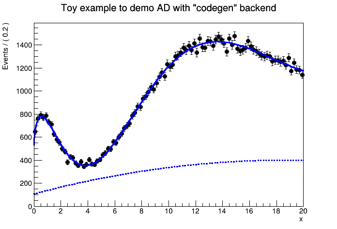
Below, you can find a little example on how to use the "codegen" backend on how to fit a simple example. Note that in this example, we only have 5 parameters, and the highly-optimized numeric gradients in default RooFit are still more performant.

RooRealVar x("x", "x", 0., 20.);

RooRealVar alpha("alpha", "alpha", 5, 0.1, 10);

RooGenericPdf genpdf("genpdf", "genpdf",
                     "1.+0.1 * abs(x)+sin(sqrt(abs(x*alpha+0.1)))",
                     {x, alpha});

RooRealVar a0("a0", "a0", 0.5, 0., 1.);
RooRealVar a1("a1", "a1", -0.2, -1., 1.);
RooChebychev bkg("bkg", "Background", x, RooArgSet(a0, a1));

RooRealVar nsig{"nsig", "nsig", 70000, 0, 100000};
RooRealVar nbkg{"nbkg", "nbkg", 30000, 0, 100000};

RooAddPdf model{"model", "model", {genpdf, bkg}, {nsig, nbkg}};

std::unique_ptr<RooAbsData> data{model.generate(x)};

model.fitTo(*data, EvalBackend("codegen"));

When plotting the model and the data, it would look like this:

Another feature that you get is the ability do dump the generated likelihood code in a macro.

You can do so as follows, but notice that the interface is experimental and might change any time:

   std::unique_ptr<RooAbsReal> nll{model.createNLL(*data, EvalBackend("codegen"))};
   static_cast<RooFit::Experimental::RooFuncWrapper&>(*nll).writeDebugMacro("debug_macro");

Some notes on performance

The basic example above does not get sped up by activating "codegen". But why? And for what kind of fits is it worth it now? As discussed before, the runtime of reverse mode AD gradients is about 6 to 7 times the runtime of the nominal function. For numeric gradients, one needs to run the function n times, where n, is the number of parameters. So one needs at least about 7 parameters for AD to pay off in runtime. However, there is one additional factor particular to RooFit: the evaluation of the nominal likelihood function is accelerated by RooFits new vectorizing computation backend (see this talk at CHEP 2023 for more detail). The vectorization gives RooFit roughly a 4x speedup for free: to split up the computations in severall vectorizable loops, RooFit needs to track intermediate results, but it needs to do so anyway for the caching. As explained earlier, the analytic gradient should not do any caching and therefore taking the same approach to vectorization-friendly code in the code generation would result in an unreasonable memory overhead. Hence, AD in RooFit only starts to get worth it for about at least 30 parameters. In cutting-edge combined analyses, this number is easily excceeded by more than an order of magnitude.

But does the speedup you get with AD in RooFit grow indefinitely with the number of parameter in the model? The answer is no, unfortunately. There are two reasons. One reason is that the caching in RooFit already alleviates the bad performance scaling of numeric gradients, at least in most cases. There is still one case where the caching is ineffective, which is when you have large user-defined formulae in your model (either via the RooGenericPdf or the RooFormulaVar). For RooFit, such user formulae are a blackbox and it cannot cache any intermediate result. This is exactly where the code generation shines! The formulae are copied as-is in the generated code, and Clad can produce maximally-optimized gradients. For such models, our uses report minimization speedups of up to 10x when using AD! The other reason for the limited speedup when using AD is Minuit2, which is based on the Broyden–Fletcher–Goldfarb–Shanno (BFGS) algorithm. The BFGS algorithm includes a numeric line search to determine the step size in each iteration, and when the gradient comes “for free”, the minimization time is dominated by the line search. The same limitation also applies to parallelizing the gradient with multiprocessing, as explained in more detail in this ICHEP 2022 presentation.

Benchmarks with large-scale combined fits

After all this discussion, let’s take a look at some benchmark with real Higgs combination fits! Such benchmarks can be found in the previously-linked ICHEP 2024 presentation. In that presentation, AD is applied to CMS Higgs boson observation statistical model, which was also released as open data in 2024. Furthermore, the presentation also shows benchmark results for an ATLAS Higgs analysis based on toy data, which can be found in the rootbench repository (the plots in that presentation show the minimization time for the likelihood in the WS-VHbb-STXS_mu_toy_new.root workspace, which combines 53 different measurement channels in a HistFactory model).

The benchmark plot for the ATLAS model was updated and improved exclusively for this blog post. Let’s take a look!

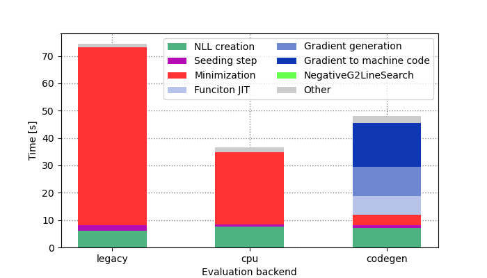
The plot compares the runtime for the full workflow of likelihood creation and minimization with the different RooFit evaluation backends, breaking down the runtime into different steps. The first message is that new RooFit vectorizing "cpu" backend gives you a 2x speedup for free in this case. On top of this, the minimization time can be further reduced by a factor of 10 when using AD via the "codegen" backend! But this comes at a cost: the overhead of compiling the generated code, generating the gradient code with Clad, and compiling the gradient to machine code is significant, and only pays off when you intend to do several minimization passes. However, optimizing this just-in-time compilation is a problem that factorizes very well from RooFit development, being mostly related to the Clad tool. Given the rapid development of Clad, we can assume that this overhead will significantly reduce with the next ROOT releases.

Summary and outlook

Using AD in RooFit with the "codegen" is very well worth it in fits with more than about 30 free parameters, because it can massively speed up the minimization. This is especially the case for models with user-defined functions in RooFormulaVar or RooGenericPdf instances. In the future, we will work on extending support in the "codegen" for more diverse RooFit models. We also strive to implement optimized Hessian evaluations using AD, such that you can benefit from much faster uncertainty estimation using the "Hesse" algorithm in Minuit2.

One ambitious plan we have for the immediate future is supporting workflows doing Simulation Based Inference (SBI). As demonstrated in this CHEP 2024 conference presentation, RooFit has already the facility to include neural networks trained with Python as part of the likelihood. Our goal is to also support neural network inference in "codegen" enabled by TMVA-SOFIE. By the end of the year, we want to have a fully-differentiable SBI demonstrator.

Stay tuned for the ACAT 2025 conference!